Linear Regression Channel Backtest on AAPL (2018–2025): The Boring Line That Survives
A 60-day linear regression channel on daily AAPL, 2018–2025: +199% total, half of buy & hold's drawdown, and — uniquely in this series — profitable in every cost scenario including 25bp slippage. The least glamorous strategy is the only cost-survivor, in pandas with charts.
Linear Regression Channel Backtest on AAPL (2018–2025, daily, real fees)
Fifteen strategies into this lab, fees have eaten everything: hourly crypto churns, and every churn pays the exchange. Then I ran the least glamorous thing on my screen — a straight line fitted through 60 days of closing prices — and it became the first strategy that survives a realistic cost model. No fancy entries, no multi-timeframe filters, no machine learning. Just OLS, on daily AAPL, for eight years. Strategy Lab #17.
What a linear regression channel is
For each bar, fit a straight line through the last 60 closes using ordinary least squares:
close_t ≈ a + b·tThe fitted line is the trend of the moment; the spread of residuals tells you how far price has wandered from it. My rule is the simple channel reading:
- Long while close > the 60-day regression line.
That's the entire strategy — 106 trades over eight years, about 13 a year. The sample is AAPL daily (2018–2025), so there's no funding cost at all; the only fees are the two taker legs per round trip.
Results
| Strategy | Category | Total return | CAGR | MaxDD | Sharpe | Trades |
|---|---|---|---|---|---|---|
| linreg | statistical | +199.09% | +22.01% | -23.34% | 1.02 | 106 |
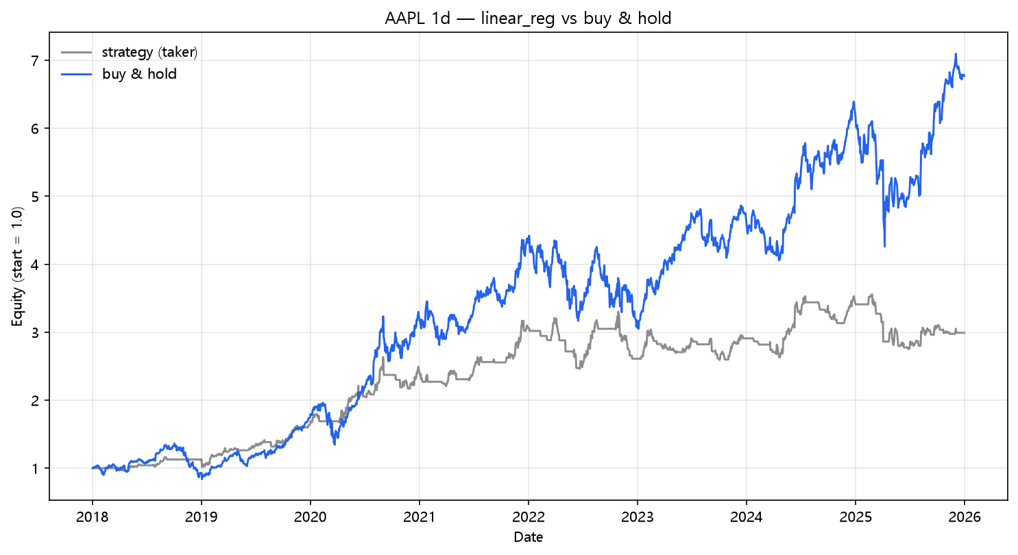
The honest-cost line is +199.09% with a -23.34% max drawdown. Now compare that to just holding the stock: buy & hold made +576.91% but lost -38.52% at its worst — and that drawdown was the 2022 bear, which people actually lived through. The regression line gets you half the return with half the pain and a nearly identical Sharpe (1.02 vs 1.12). That's the trade the chart is offering: less money, more sleep.
Every cost scenario is positive
| Scenario | Cost/leg | Total return | MaxDD | Sharpe | Trades | |---|---|---:|---:|---:|---:|---:| | naive (zero cost) | 0.00% | +232.54% | -22.96% | 1.11 | 106 | | taker fee 0.05%/leg | 0.05% | +199.09% | -23.34% | 1.02 | 106 | | + funding 0.01%/8h | 0.05% | +199.09% | -23.34% | 1.02 | 106 | | + slippage 10bp/leg | 0.15% | +141.90% | -24.77% | 0.84 | 106 | | + slippage 25bp/leg | 0.30% | +75.88% | -34.53% | 0.58 | 106 |
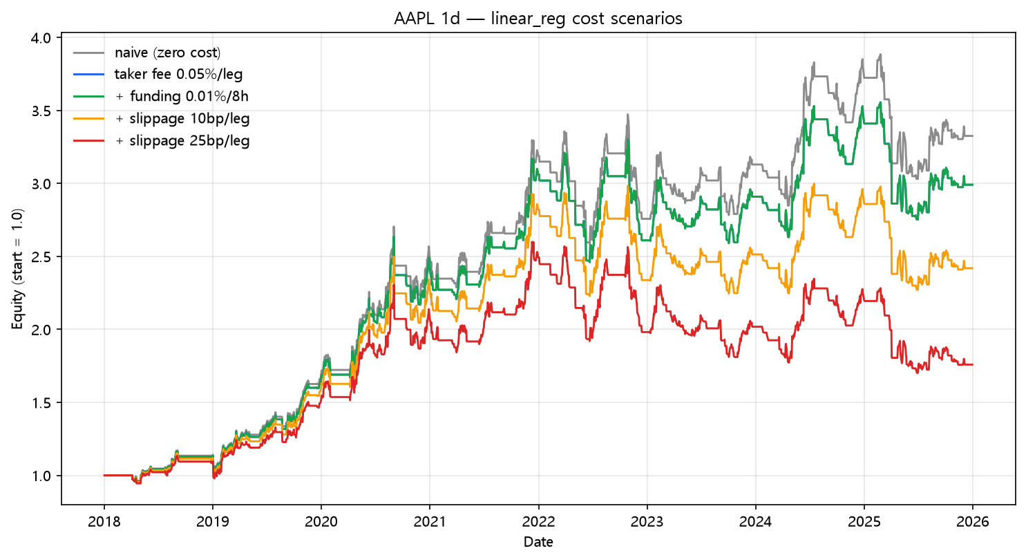
Every row is green. Not because the indicator is magic, but because it trades 13 times a year instead of 700. Compare with OBV (#16): identical logic (series above its own trendline), 106 trades vs 734, +75.88% vs -98.10% at the same 25bp cost. The difference is frequency, not foresight. This is the single most important number in the whole series, and it's the trade count.
Buy and hold comparison
| Strategy | Total return | CAGR | MaxDD | Sharpe |
|---|---|---|---|---|
| linreg | +199.09% | +22.01% | -23.34% | 1.02 |
| buy & hold | +576.91% | +41.52% | -38.52% | 1.12 |
What this does NOT prove
- A fitted line is not a prediction. The regression channel describes the past 60 days; it has no opinion about tomorrow. What made it survive is that it stays in stocks that are above their own trend and leaves before the drawdown deepens — a trend filter, not a crystal ball.
- One very strong stock, eight years, daily bars. AAPL has an excellent 2018–2025; the same channel on an index or a different decade will differ. What survives a regime change is the low-frequency principle, not the 60-day parameter.
- This is the setup for the last post in the lab (#18): statistical signals on daily data are the one branch that holds up under costs — so the next step, machine learning, should start here, not on hourly crypto.
Code
from backtest_base import fetch, backtest_signal, metrics
import numpy as np

df = fetch("AAPL", "yahoo", "2018-01-01", "2025-12-31", "1d")
close = df["close"]
t = np.arange(len(close))

def reg(ts):                       # OLS fit over a 60-bar window
    x = ts[-60:]
    slope, intercept = np.polyfit(np.arange(60), x, 1)
    return intercept + slope * 59  # line value at the last bar

line = close.rolling(60).apply(reg, raw=True)
signal = (close > line).fillna(False)
res = backtest_signal(df, signal, cost_per_leg=0.0005, funding_per_bar=0.0)
print(metrics(res, 365))
Reproduce it
cd blog-drafts/scripts
python backtest_base.py --strategy linear_reg --symbol AAPL --interval 1d \
    --start 2018-01-01 --end 2025-12-31 --fee 0.0005 --funding 0
Data: Yahoo Finance, daily OHLCV, 2,010 bars. The tables above reproduce exactly from this command.
This is a backtest on historical data, not investment advice. Past performance does not predict future results.