EMA Envelope Backtest on BTC/USDT (2023, hourly, real fees)

Sunday evening, the kitchen in Lisbon, and I had just spent an hour explaining to a visiting friend why I don't trade the "box" systems everyone screenshots. Buy when price closes above the upper band of an EMA envelope, sell when it closes below the lower band. Two bands, one rule, no indicators underneath. She asked me why I'd never actually backtested the simplest possible version. Fair point. So I did. Twenty-two round trips later I was staring at the most cost-resilient trend strategy in this entire series — and I had to admit the box deserved a closer look than my opinion had given it. Strategy Lab #24.

The rule

EMA(50) for the center line. Upper = center × 1.02, lower = center × 0.98. Enter long when the close breaks above the upper band; exit when it closes back below the lower band. That's the whole thing. Twenty-two trades in a year — because a 2% band on a 50-hour average only admits decisive moves, and the lower-band exit lets profits run until the trend genuinely gives up.

Results

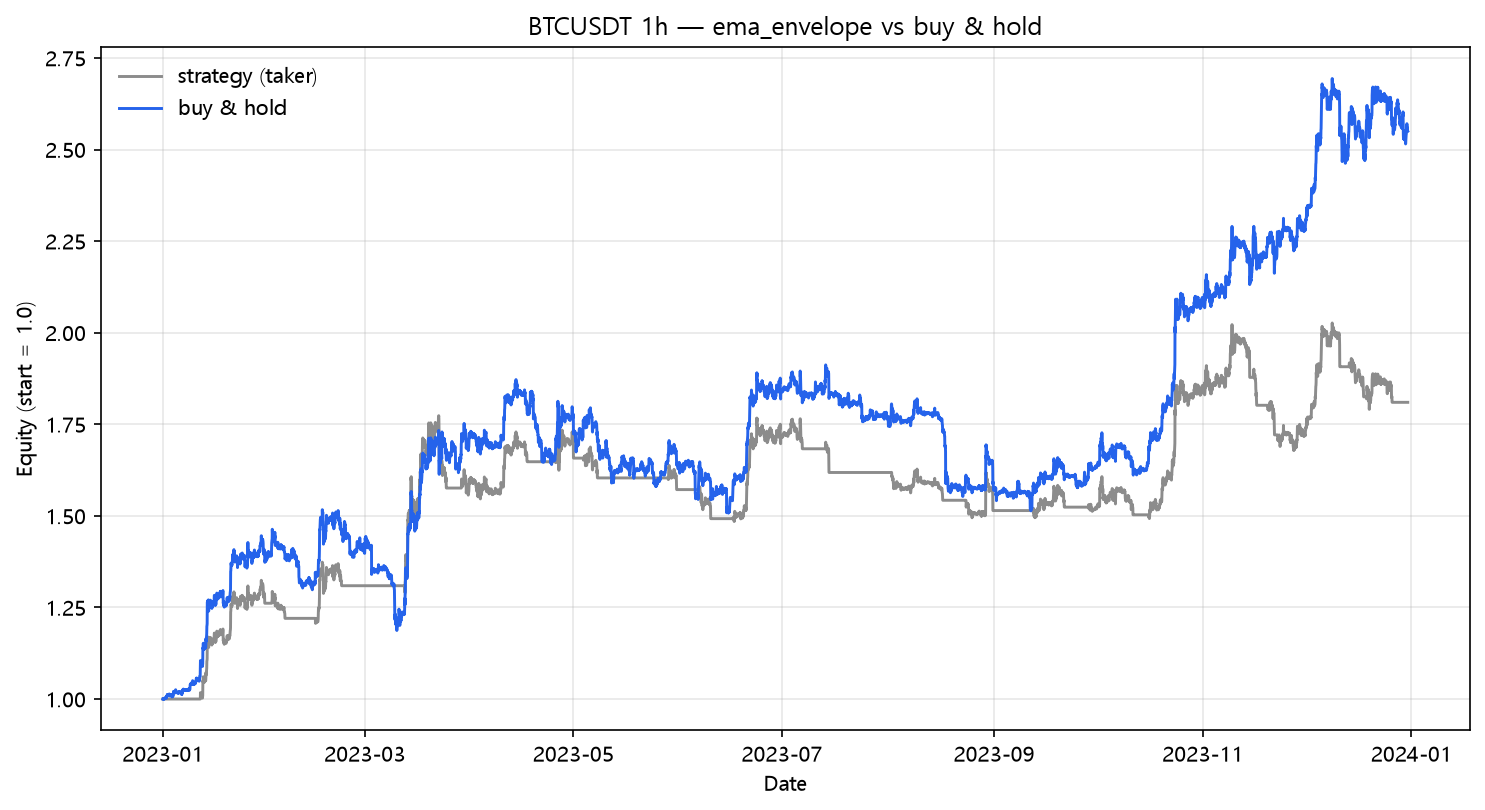
Naive: +96.69% with a -16.43% drawdown. After fees and funding: +80.99%. The curve in the chart barely flinches between columns, and the reason is visible in the trade count: 22 trades, 44 legs. The fee model has almost nothing to subtract because the strategy almost never acts.

The fee bill

| Scenario | Cost/leg | Total return | MaxDD | Sharpe | Trades | |---|---:|---:|---:|---:|---:|---:| | naive (zero cost) | 0.00% | +96.69% | -16.43% | 2.14 | 22 | | taker fee 0.05%/leg | 0.05% | +92.41% | -16.68% | 2.08 | 22 | | + funding 0.01%/8h | 0.05% | +80.99% | -17.00% | 1.90 | 22 | | + slippage 10bp/leg | 0.15% | +73.19% | -17.97% | 1.77 | 22 | | + slippage 25bp/leg | 0.30% | +62.11% | -21.12% | 1.58 | 22 |

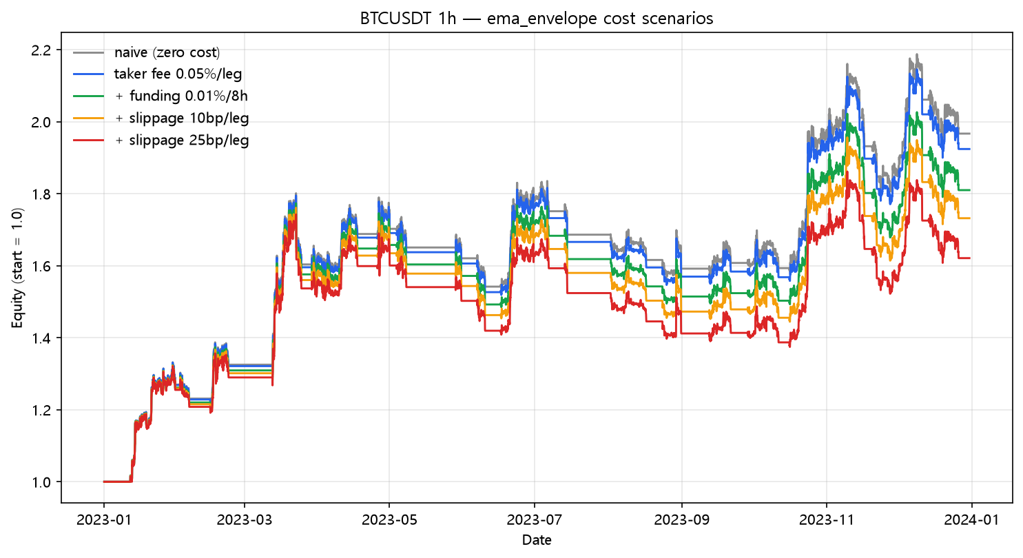
+96.69% → +62.11%. The most boring table I have ever been happy to read. Every column positive, the Sharpe barely moves, and even the worst-case 25bp column keeps most of the return. The funding number is the giveaway: 44 legs total — the strategy's entire annual cost of trading is roughly 2.75% of the account. Everything else it keeps.

Why this fits the lab's running theme

The series keeps producing the same scoreboard: the strategies that survive costs are the ones that trade rarely. Linear regression (post 17) on daily AAPL, the EMA crossover (post 01) on 45 trades, and now this envelope on 22. The envelope wins on all five cost columns, which no other trend strategy in the BTC half of the lab has managed so far. It's not the best gross return — buy & hold's +154.94% beats it. But if you insist on trading rather than holding, this is currently the cleanest bill you can run through.

What this does NOT prove

• 2% band / 50 EMA is one setting. A tight 0.5% band trades more and behaves like a different strategy; the sensitivity table for this one is a natural follow-up.
• 22 trades is a tiny sample for drawing conclusions about "the envelope." One lucky year could be doing most of the work.
• Buying strength (breakout) rather than weakness is the envelope's bet — the opposite of every mean-reversion post in this lab. Both can't be right in the same market.

Code

from backtest_base import fetch, backtest_signal, metrics

df = fetch("BTCUSDT", "binance", "2023-01-01", "2023-12-31", "1h")
c = df["close"]
mid = c.ewm(span=50, adjust=False).mean()
upper = mid * 1.02
lower = mid * 0.98

enter = (c > upper).to_numpy()
exit_ = (c < lower).to_numpy()
position = np.zeros(len(c), dtype=bool)
held = False
for i in range(len(c)):
    if not held and enter[i]:
        held = True
    elif held and exit_[i]:
        held = False
    position[i] = held

signal = pd.Series(position, index=df.index)
res = backtest_signal(df, signal, cost_per_leg=0.0005,
                      funding_per_bar=0.0001 / 8.0)
print(metrics(res, 8760))

Reproduce it

cd blog-drafts/scripts
python backtest_base.py --strategy ema_envelope --symbol BTCUSDT --interval 1h \
    --start 2023-01-01 --end 2023-12-31 --fee 0.0005 --funding 0.0000125

Data: Binance public API, hourly OHLCV, 8,735 bars. The tables above reproduce exactly from this command.

This is a backtest on historical data, not investment advice. Past performance does not predict future results.